In this post, I will discuss the connection between the perceptron grokking scenario (discussed in a previous post) and the problem of learning local rules. Concretely, I will discuss a mapping from a sequence-to-sequence rule learning problem to a simple binary classification (grokking) task. I will also compare the numerical simulations with the predictions of the perceptron grokking model discussed in a previous post.

Details can be found in arXiv:2210.15435.

Motivation: statistical learning vs. grokking

The simplest and probably most studied (rule) learning scenario is the teacher-student learning paradigm, where we consider two perceptron models with $N$ binary inputs and one binary output. The first network is a teacher determining the rule, and the second is a student, which we train on a certain number of input-output pairs determined by the teacher. Our task is to find a student model that best reproduces given training data. The main goal of the learning theory is to determine the generalization properties of the trained student model. Commonly we measure generalization in terms of the fraction of incorrect outputs (the generalization error). It is, however, not trivial to see how a trained student model generalizes to unseen teacher-generated pairs. We typically study generalization with statistical-mechanics methods and consider the thermodynamic limit, i.e., we take the limit of infinitely large models $N\rightarrow\infty$. Without further restrictions, we can show (and it is intuitively clear) that the generalization error will decrease continuously with the number of updates but will not reach zero in a finite number of steps. Concretely, the generalization error decays algebraically with the number of samples.

Fast forward to deep neural networks. Recently an intriguing phenomenon has been observed in training deep neural networks on algorithmic datasets. After a zero training error has been achieved, a transition to zero test/generalization error from almost one to zero has been observed and named grokking by A. Power et al.).

The observation of a transition to zero generalization error at a finite time can not be explained by the standard statistical learning theory (without any phase space restrictions). A simple explanation of grokking is offered by perceptron grokking model. However, it is not trivial to connect the perceptron grokking setup with the standard learning theory. In the following, I will describe precisely this connection using a tensor-network attention model.

Local rules and tensor network attention

We will consider a particular teacher-student problem, the sequence-to-sequence learning problem on binary sequences. We further restrict the transformations such that the value of the output sequence at position $i$ depends only on $2K+1$ values of the input

$y_i=\mathrm{rule}(x_{i-K},x_{i-K+1},\ldots x_i,\ldots x_{i+K}).$

In other words, we define the teacher by a $K-$local rule, which can be contrasted with the standard statistical learning scenario, where the rule is infinite range. The input and the output sequence have the same length $M$, which can be arbitrary.

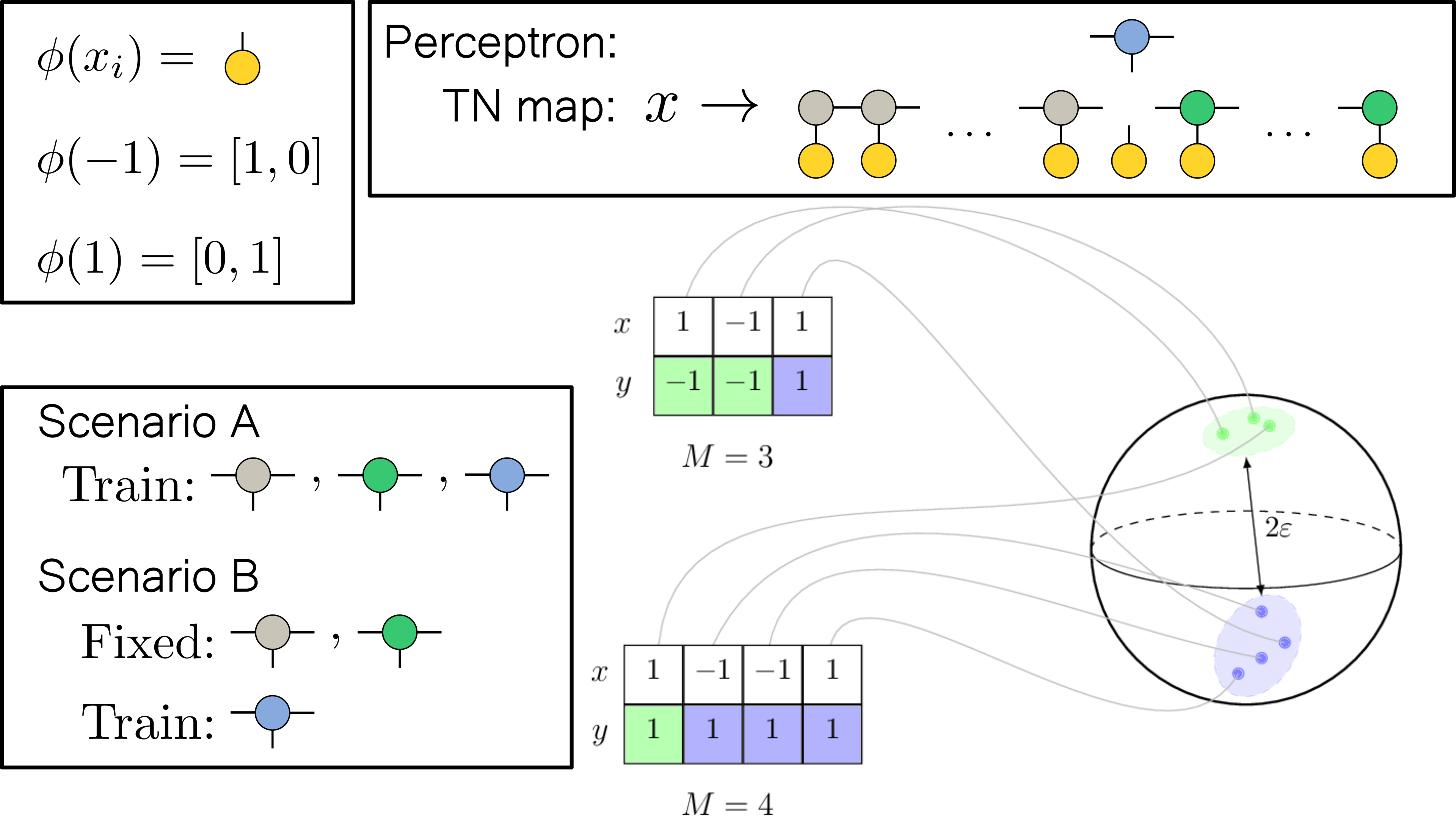
Our task is to learn the rule on a finite number of training samples. For that, we first need to define a student model. We need to consider a student model class that can handle variable-size inputs. The standard model choice in this regard is a recurrent neural network. We, however, will use a uniform tensor-network attention model. Actually, we can interpret tensor-network attention as a particular recurrent neural network. The simplest way to represent the tensor network architecture is by using diagrammatic notation. The image below shows the model output at position $i$ before the final sign non-linearity.

The gray/green tensors represent the left/right context tensors, the blue tensor is a classification tensor, and the orange tensors represent the local embeddings defined as

$\phi(0)=[1,0],\quad \phi(1)=[0,1].$

We will consider two scenarios:

• Scenario A: All tensor-network attention tensors are trainable
• Scenario B: We fix the context tensors and train only the classification tensor

From sequence-to-sequence learning to perceptron grokking

Before continuing to the results, I will introduce another interpretation of the model. We can interpret the tensor-network attention model without the (blue) classification tensor as a map from a $[0,1]^M$ binary input sequence to a $2D^2$ real vector space which is independent of the sequence length $M$.

In this picture, the context part of the tensor-network attention layer embeds the (possibly infinite) input sequence into a finite-dimensional vector space. We can interpret the classification tensor in this space as a perceptron model. Therefore, we have transformed the sequence-to-sequence learning problem into a (grokking) perceptron binary classification problem.

In the following, I will describe the results of training the tensor-network attention model (scenarios A and B).

Training only the classification tensor (scenario B)

Comparison with perceptron grokking

I will first discuss scenario B, where we train only the classification tensor. Here we assume, that the initial context tensors are chosen such, that the obtained binary classification problem is solvable/linearly separable. We can calculate the generalization-error critical exponent $\nu$, the effective dimension $D_{\rm eff}$, the divergence of the data distribution at the domain boundary $\xi$, and the class separation $\epsilon$ numerically for different realizations of the context tensors. Then we can check the predictions of the $D$-dimensional-ball perceptron-grokking model from arXiv:2210.15435. Indeed we find that the simple perceptron grokking predicts the relation between the quantities $\nu,\xi$, and $D_{\rm eff}$ relatively well.

We also find that the bimodal structure of the grokking time probability density function predicted by the perceptron grokking model is reproduced in the local rule learning scenario.

Training the full tensor-network attention model

Structure formation

By training the context tensors we change the positive and negative feature space data distributions. This enables us to observe feature space structure formation, which we can detect as a sharp drop in the average effective dimension over many different initial conditions.

For a small enough bond dimension, we can directly observe the training data distribution during training. An example with bond dimension three is shown below.

The figure above shows two training runs. The gray lines in the left panels correspond to training without regularization, and the orange lines correspond to training with L1 regularization. The right panels correspond to the feature space data distribution at different times (top: regularized case, bottom: non-regularized case). The regularized case attains zero generalization error quicker than the non-regularized case. However, regularization increases the number of spikes in loss. Therefore, it seems beneficial to start with a large regularization and then reduce it to avoid loss spikes. The spikes are associated with structural changes. In the right panels, we can see that structural changes may persist after the spikes, which we can detect by a step-like behavior in the effective dimension.

Takeaway

• A local sequence-to-sequence prediction task in the thermodynamic limit can be transformed into a classification problem on a finite domain.
• The obtained classification problem is well described by the perceptron grokking model.
• Spikes in the training loss correspond to latent space structural changes in the training data.
• Regularization reduces the average effective dimension of the feature space data, leads to faster grokking, but increases the frequency of training loss spikes.
• Strong regularization seems beneficial at the early stages of training but not at the late stages.
• Many unanswered questions: Why are spikes in the training loss periodic? Why does the spike frequency increase with larger regularization? What exactly is the mechanism of the structural changes (corresponding to training loss spikes)? How does grokking look for more complicated rules? What is the role of symmetries and conservation laws in grokking and rule learning in general? And more...