What is grokking?

Grokking has been observed by A. Power et al., and it refers to the "sudden" transition of the test/generalization error from almost one to zero. Moreover, this transition typically happens long after we reached zero training error.

The above figure is the main observation of the paper by A. Power et al. and shows that optimizing the network beyond zero training error can have a significant effect on the generalization error. Moreover, the transition to a high generalization accuracy is not gradual but "sudden" (at least in the log scale :) ). In this post, I will present a simple perceptron grokking model, that features the observed phenomenon and is amenable to an exact analytic solution. In the next post on tensor-network grokking, I will discuss the relevance of the perceptron grokking model in the rule learning scenario.

Perceptron grokking

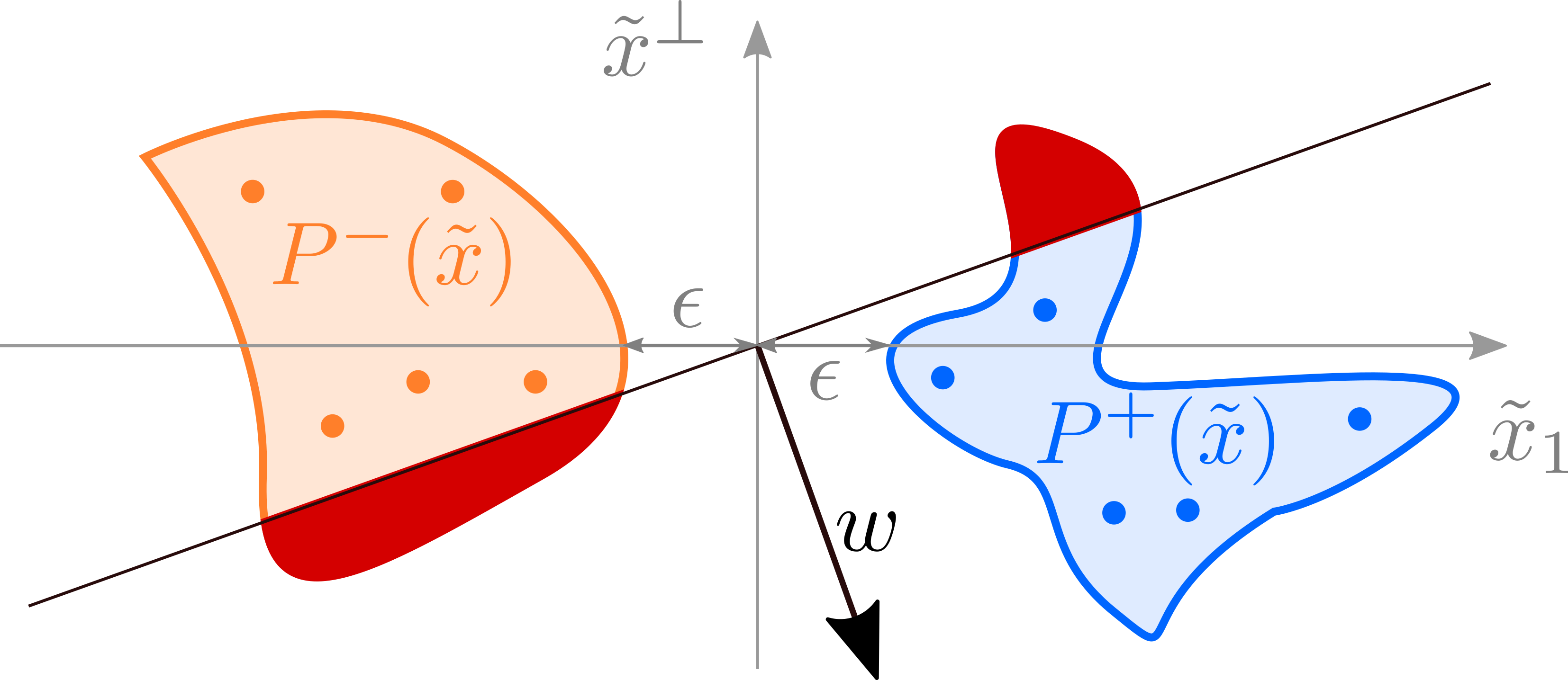
I will focus on the first part of the perceptron grokking model introduced in arXiv:2210.15435, which contains all main features though it is perhaps not directly applicable in practice. The primary motivation for the model was to develop a simple, possibly analytically tractable model, which shows a similar behavior as in the figure above. The easiest setup/problem I could imagine is the binary classification with a perceptron, which is sufficient to describe the grokking phenomenon. I will assume that the positive and the negative data distribution are linearly separable and denote the distance between the two distributions by $2\varepsilon$. Our task will be to train a perceptron model with gradient descent (full batch training) and analyze the generalization error. A schematic representation of the setup is presented in the figure below.

The blue region encompasses all positive data, and the orange one all negative data. The dots represent training samples. The current model is determined by the vector $w$ and correctly classifies all training samples. In contrast, the generalization error is given by the "area" of the red region. By continuing training (e.g. minimizing the MSE), we eventually end up with a model with zero generalization error. Therefore, by construction, our simple model features all phenomena observed by A. Power et. al. The main task now is to explicitly define the probability distributions of positive and negative data and calculate the generalization error.

In the paper, we discuss two distributions:

• 1D exponential distribution: (pros) can be solved analytically and contains most qualitative features observed in the second distribution, (cons) can not be quantitatively compared with the experiments
• D-dimensional uniform ball distributions: (pros) applies to the transfer learning and the local-rule learning setting, (cons) relatively heavy calculations, many approximations, solutions not in closed form.

Below I will explain in detail the derivation for the first/exponential distribution and highlight the main points in bold at the end of each section.

Exponential distribution

The simplest possible case we can consider is the 1D-perceptron model with exponentially distributed positive and negative samples, as shown in the figure below.

The model $\hat{y}(x)=\mathrm{sgn}(x-b)$ is given by the position $b$ and shown as a vertical line, and the generalization is given by the interval highlighted with blue. Our task will now be to describe the evolution of the generalization error during training (the length of the highlighted interval). For simplicity, we will use a dataset of $2N$ random samples ($N$ positive and $N$ negative). We also include the L1 and L2 regularization to study their effect on generalization. Our final loss, which we will optimize with gradient descent, is

$\mathcal{R}=\frac{1}{2N}\sum_{i=1}^{2N}\frac{1}{2}((\tilde{x}^i-b)-y^i)^2+\frac{\lambda_2b^2}{2}+\lambda_1 |w|.$

Since we have an equal number of positive and negative samples, we have $\sum_{i=1}^{2N}y^i=0$. We optimize our loss by integrating the gradient descent equation

$\frac{\partial b}{\partial t}=-\frac{\partial \mathcal{R}}{\partial b}=\bar{x}-\mathrm{sgn}(b)\lambda_1-(1+\lambda_2)b,$

where $\bar{x}=\frac{1}{2N}\sum_{i=1}^{2N}\tilde{x}^i$. The solution to the equation above is

$b(t)= \bar{x}_\lambda-\left(\bar{x}_\lambda-b(0)\right)\mathrm{e}^{-(1+\lambda_2)t},\quad \bar{x}_\lambda=\begin{cases} \frac{\bar{x}-\lambda_1}{1+\lambda_2}, & b(t)\geq 0\\ \frac{\bar{x}+\lambda_1}{1+\lambda_2}, & b(t)<0 \end{cases},$

and evolution of the generalization is then given by

$E(t)=\begin{cases} \frac{1}{2}(1-\mathrm{e}^{\epsilon-b(t)})& b(t)>\epsilon \\ 0 &{\rm else}\end{cases}.$

The model parameter $b(t)$ converges exponentially towards its final value $b(t=\infty)=\bar{x}$. The generalization error vanishes iff $b(t)\leq\epsilon$.

Critical exponent

The generalization error vanishes if $b(t)<\epsilon$, which happens at time

$t_\epsilon = \log\left(\frac{b(0)-\bar{x}_\lambda}{\epsilon-\bar{x}_\lambda}\right).$

To find the critical exponent, we expand around the time $t_\epsilon$

$E(t<t_\epsilon)\approx \frac{(\epsilon-\bar{x}_\lambda)}{2}(1+\lambda_2) (t_\epsilon- t).$

The above formula is valid for any initial condition with $b(0)>\epsilon$. We can now average over initial conditions with $b(0)>\epsilon$ by first aligning the time evolutions at $t_\epsilon$ and then averaging the generalization error. We find

$E(t)\rangle\rangle\approx\frac{\epsilon_\lambda}{2}(t_\epsilon-t),\quad \epsilon_\lambda=\epsilon(1+\lambda_2)+\lambda_1,$

where $\langle\langle \bullet\rangle\rangle$ denotes the average over all valid initial conditions $b(0)$ and training input averages $\bar{x}$.

Grokking in the considered 1D exponential model is a second-order phase transition at a finite time with the generalization-error critical exponent equal to one.

Grokking probability

What is the probability of grokking if we train on $2N$ random samples from the exponential probability distributions? Does this probability depend on the choice of the initial condition or the training/regularization parameters (L1 and L2 regularization strengths)? In the case of 1D exponential distributions, we can answer these questions analytically in closed form.

First, we rewrite the condition for grokking as

$|\bar{x}|<\epsilon_\lambda$

The probability of sampling a training dataset with the average $\bar{x}$ is given by

$P_N(\bar{x})=\int_{\bar{x}_+=0}^{\infty}\mathrm{d}\bar{x}_+P_N^{\rm exp}(\bar{x}_+)\int_{\bar{x}_-=0}^{\infty}\mathrm{d}\bar{x}_-P_N^{\rm exp}(\bar{x}_-)\delta\left(\bar{x}-(\bar{x}_+-\bar{x}_-)/2\right)$

$P_N(\bar{x})= \frac{2 N^{N+\frac{1}{2}} \bar{x}^{N-\frac{1}{2}} K_{N-\frac{1}{2}}(2 N \bar{x})}{\sqrt{\pi } \Gamma (N)},$

where $P_N^{\rm exp}(\bar{x})$ is a probability of sampling $N$ independent instances (from an exponential distribution), which have the average $\bar{x}$. The $K_n(z)$ is the modified Bessel function of the second kind.

The probability of sampling a dataset with zero generalization error is then given by

$P_{E(\infty)=0}(\epsilon_\lambda,N)=2\int_{\bar{x}=0}^{\epsilon_\lambda}P_N(\bar{x})\mathrm{d}\bar{x}$

${\small P_{E(\infty)=0}(\epsilon_\lambda,N)=\sqrt{\pi } (-1)^N (B \epsilon_\lambda )^{2 N} {}_1\tilde{F}_2\left(N;N+\frac{1}{2},N+1;N^2 \epsilon_\lambda ^2\right) +\frac{\pi (-1)^{N+1} N \epsilon_\lambda {}_1\tilde{F}_2\left(\frac{1}{2};\frac{3}{2},\frac{3}{2}-N;N^2 \epsilon_\lambda ^2\right)}{\Gamma (Nd)},}$ where ${}_p\tilde{F}_q\left(a;b;z\right)$ is the regularized generalized hypergeometric function.

For a particular choice of $N$, the final equation simplifies. In the case $N=2$ we have

$P_{E(\infty)=0}(\epsilon_\lambda,N=2)=1-(1+2\epsilon_\lambda)\mathrm{e}^{-4\epsilon_\lambda}.$

The final expression is nice since it gives us an exact handle on the regularization effect on generalization.

The effect of the $L_1$ and $L_2$ regularization on the trained model is different. The $L_2$ regularization is multiplicative, and the $L_1$ regularization is additive concerning the gap between the positive and negative samples $\epsilon$. Hence, in the case of a small gap, the $L_1$ regularization becomes much more effective. We also find a similar distinction between the $L_1$ and $L_2$ normalized models in the more general grokking scenario.

L1-regularization is preferred to L2-regularization. In case of an infinitesimal gap ($\epsilon\ll1$) and finite $N$, the $L_1$ regularization ensures that the probability of zero generalization error is finite. In contrast, the grokking probability vanishes for any value of the $L_2$ regularization. We observe the same behavior also in the $D-$dimensional ball setting.

Grokking time

The last quantity we calculated in the paper was the grokking-time probability density function. I will omit the calculation here since it is not instructive and the findings do not generalize to the more complicated case. Instead, I will show several exact evaluations of the grokking-time probability density function at the different effective separations between classes $\epsilon_\lambda$.

The above figure shows numerically exactly the grokking-time $t_{\rm G}$ probability density function at a different number of training samples $N=$2 (dashed blue line), 5 (dotted orange line), 10 (full green line). The panels correspond to $\epsilon_\lambda=$0.4 (left), 0.04 (middle), 0.004 (right). As expected grokking time is shorter with increasing $N$ and $\epsilon_\lambda$.

More training samples and larger effective class separation lead to shorter mean grokking time.

Takeaway

1. We can explain grokking with a perceptron model.

2. L1 and L2 regularization have a qualitatively different effect on generalization. The L1 regularization increases the effective class separation additively. In contrast, the L2 regularization increases the class separation multiplicatively.

The generalization to non-separable distributions is a work in progress.