The first tansor network approach that achieved the state-of-the-art (SOTA) result in a machine learning task was the anaomaly detection approach of Wang et al. I will describe a generalization of the approach to the positive unlabeled learning problem. The resulting model achieves the current SOTA for the PUL problem on categorical datasets as well as on the MNIST image dataset.

You can find more in the original paper "Positive unlabeled learning with tensor networks." Neurocomputing 552 (2023): 126556. A basic implementation is available on git.

Model overview

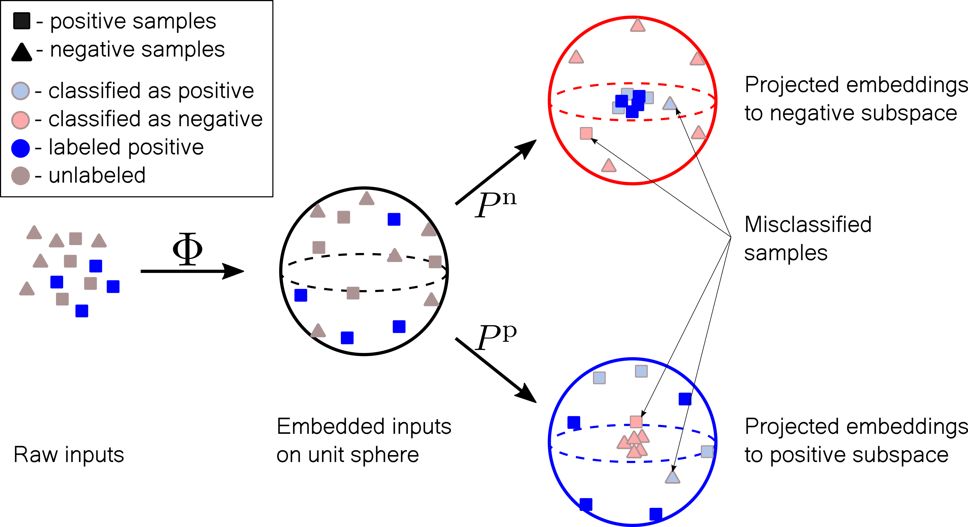
The idea of the model is depicted in the figure below. We first embed the input $x$ in an exponentially large (in the size of the vector) vector space. we can separate the positive and negative datasets with a linear map, if the embedding is sufficiently expressive. In addition, we want to find a good representation of the probability distributions of the positive and negative embedded samples. To achieve both goals we project the embedded data with two projectors. The positive projector will project the positive instances onto a sphere of radius one and the negative instances into the origin of the sphere. In contrast, the negative projector will project the negative instances onto a sphere of radius one and the positive instances to the origin.

The projections therefore determine positive and negative subspaces in the embedding space. Therefore, they can be interpreted as an approximation of the square roots of the embedding space probability distributions of the positive and negative samples. Finally, the tensor network structure of the approximate probabilitiess enables efficient unbiased sampling.

Workflow

The entire production workflow of the proposed tensor network model is summarised as follows.

1. Flatten If the input is multi-dimensional, we flatten it such that the first dimension is the batch dimension and the second is the feature dimension. We use N to determine the number of features. After flattening the working tensor if of size $n_{\rm bath}\times N$, where $n_{\rm bath}$ determines the batch size.

2. Normalization We normalize the data to the domain of the embedding map. We use an embedding with a unit interval domain for each feature. Hence we normalize all features to the unit interval. Categorical features are first represented as integers and then normalized.

3. Embedding We transform each feature by an embedding function, which may vary for different features. However, we use the same embedding function for all features. The embedded tensor has dimension $n_{\rm bath}\times N\times d$, where $d$ is the dimension of the local embedding.

4. Log-norm Finally, we calculate the norms of positive and negative projections by contracting the embedding tensor with the LPS tensor networks. To avoid numerical overflow, we calculate the log-norm of the positive and negative projections. The class is positive if the log norm of the positive projection is larger than the log-norm of the negative projection.

Embedding transformation

Let'w check how the embedding transformation works. A tensor-network embedding transforms the raw data (numerical or categorical) to a real or complex Hilbert space. The embedded data is typically represented as a product state in the large Hilbert space. We reughly distinguish two types of embeddings, quantum and probabilistic. In the first case, the embedding is always $L2$ normalized, can be interpreted as a quantum state, and implemented on an actual quantum device. In the probabilistic case, the embedding functions need to be orthonormal over the attribute domain. The orthonormality enables efficient normalization of the probability (or calculation of the partition function) by replacing the integrals over the domain variables with efficient tensor-network contractions. In our case we will use the following probabilistic embedding

$\Phi(x)=\phi(x_1)\otimes\phi(x_2)\otimes\ldots \otimes\phi(x_N), \quad \phi(x_i)=(1,\cos(\pi x)\ldots \cos((d-1)\pi x)),$

where $d$ determines the local Hilbert space dimension. Assuming that the input domain is the unit interval $x_i\in[0,1]$ it is not difficult to check that the basis functions obey the orthonormality relation

$\int_0^1\mathrm{d}u \phi_i(u)\phi_j(u)=\delta_{i,j}.$

Tensor network projectors

Let's now look how can we construct projectors acting in the exponentially large Hilbert space. The to restrict the number of parameters we encode the projectors with tensor-networks. We follow Wang et al. and use the locally purified state (LPS) tensor network.

The benefit of the LPS tensor network is that the input and the output spaces have different dimensions. This ensures that the projectors has a large kernels, that can accommodate the opposite class distributions. The corresponding same-class distribution is then given by the Cholesky product of the projectors. We calculate the norm of $\hat{y}$ associated with an LPS by contracting the following tensor network

Loss

The loss having five different terms is rather involved. However it has a nice probabilistic interpretation, which we will recall here. For details please refer to the original paper.

• First term: The first summand in $\mathcal{L}_{1}$ proportional to $\lambda_1$ minimizes the Kullback-Leibler (KL) divergence between the positive-labeled data distribution and the (positive) tensor-network approximation $\hat{y}^{\rm p}$. In contrast, the second summand in $\mathcal{L}_1$ maximizes the KL divergence between the positive-labeled data and the (negative) tensor-network approximation $\hat{y}^{\rm n}$.

• Second and third term: Similar interpretations have the second and third loss term $\mathcal{L}_2$ and $\mathcal{L}_3$: we increase the KL divergence between the opposite-class distributions and decrease the KL divergence between the same-class distributions.

• Fourth term: The fourth term normalizes the positive/negative tensor-network distributions and captures the remaining parts of the KL divergence in the losses $\mathcal{L}_{1-3}$.

• Fifth term: The final, fifth loss $\mathcal{L}_5$ ensures that the positive and negative tensor-network distributions have the same distance (KL divergence) to the uniform distribution on the unlabeled data. We can incorporate prior information into our objective by changing the uniform prior in the fifth loss $\mathcal{L}_5$ with another distribution.

Results

We tested our approach on three synthetic point datasets, the MNIST image dataset, and 15 categorical/mixed datasets. Let's look at the performance on each of them.

Synthetic datasets

The three point datasets, namely the two moon dataset, the circles dataset, and the blobs dataset available through the scipy API were used to test the generative properties of our approach. For model and training details see the manuscript. Below we show samples generated by an ensemble of four LPS models. We show the two moon dataset, blobs dataset, and circles dataset. The top panels show the training dataset, where gray denotes the unlabeled samples and blue the labeled positive samples. The bottom panels show the generated samples, where orange circles are accepted positive samples, blue circles are accepted-negative samples, and gray and red dots are rejected negative and rejected positive samples. Visually, it is clear that our method better reproduces the original distribution (especially after thresholding) when compared to the state-of-the-art GAN results.

MNIST

The state-of-the-art approaches to the PUL problems on image datasets are GANs. Hence we are comparing the performance of our model on the MNIST dataset with the performance of the best GAN approaches:

• Generative positive and unlabeled framework (GenPU): a series of five neural networks: two generators and three discriminators evaluating the positive, negative, and unlabeled distributions.

• Positive GAN (PGAN): Uses the original GAN architecture and assumes that unlabeled data are mostly negative samples.

• Divergent GAN (DGAN): Standard GAN with the addition of a biased positive-unlabeled risk. DGAN can generate only negative samples.

• Conditional generative PU framework (CGenPU)4: Uses the auxiliary classifier GAN with a new PU loss discriminating positive and negative samples. We use the trained generator network to generate training samples for the final binary classifier (two-stage approach).

• Conditional generative PU framework with an auxiliary classifier (CGenPU-AC): The same as CGenPU, but uses an additional classifier to classify the test data (single-stage approach).

Althought the LPS tensor network does not take into account the 2D structure of the image it performs significantly better as the GAN approachs even with a smaller number of labeled samples. This is the first pure tensor network model that outperforms neural netrowk models on an image related tasks.

N_p	PGAN	D-GAN	GenPU	CGenPU	CGenPU-AC	TN
100	0.69 ± 0.23	0.77 ± 0.22	0.86 ± 0.12	0.87 ± 0.19	0.89 ± 0.18	0.99 ± 0.01
10	0.60 ± 0.22	0.60 ± 0.22	0.59 ± 0.12	0.79 ± 0.21	0.84 ± 0.18	0.98 ± 0.04
1	0.84 ± 0.18	0.84 ± 0.18	0.59 ± 0.14	0.71 ± 0.25	0.72 ± 0.23	0.90 ± 0.20

Categorical and mixed data

The results on the synthetic and MNIST datasets are encouraging since we expect even better results on categorical datasets, where neural-networks typically struggle. The best performing methods on categorical data are the following:

• Positive Naive Bayes (PNB): Calculates the conditional probability for the negative class by using the prior weighted difference between the attribute probability and the conditional attribute probability for the positive class.

• Average Positive Naive Bayes (APNB): Differs from PNB in estimating prior probability for the negative class. PNB uses the unlabeled set directly, while the APNB estimates the uncertainty with a Beta distribution.

• Positive Tree Augmented Naive Bayes (PTAN): Builds on PNB by adding information about the conditional mutual information between attributes $i$ and $k$ for structure learning.

• Average Positive Tree Augmented Naive Bayes (APTAN): Differs from PTAN in estimating the prior probability for the negative class. PTAN uses the unlabeled set directly, while the APTAN estimates the uncertainty with a Beta distribution.

• Laplacian Unit-Hyperplane Classifier (LUHC): A biased PUL technique that determines a decision unit-hyperplane by solving a quadratic programming problem.

• Positive Unlabeled Learning for Categorical datasEt (Pulce) approach: A two-stage PUL approach that uses a trainable distance measure called Distance Learning for Categorical Attributes (DILCA) to find reliable negative samples. In the second stage, a k-NN classifier is used to determine the class.

• Generative Positive-Unlabeled (GPU) approach: Learns a generative model, typically using probabilistic graphical models (PGMs), from labeled positive samples. Reliable negative samples are determined as those with the lowest probability given by the trained generative model. Finally, a binary classifier, typically a support vector machine, is trained on labeled positive and reliable negative samples. This approach has also been extended by aggregating many PGMs in an ensemble.

We test all approaches on 15 categorical datasets with 30%, 40%, and 50% of positive and labeled data, which amounts to 45 different tasks. As we can see from the table below our TN approach outperforms all other approaches on the majority of the datasets and significantly improves the classification SOTA on the categorical PUL task.

Dataset	%	PNB	PTAN	APNB	APTAN	Pulce	LUHC	GPU	TN
#wins		4	0	5	0	4	6	8	32
Avg. F1 (All)		0.68	0.66	0.68	0.64	0.76	0.63	0.81	0.90
Avg. F1 (30%)		0.66	0.64	0.66	0.64	0.74	0.58	0.80	0.89
Avg. F1 (40%)		0.69	0.65	0.68	0.65	0.76	0.65	0.80	0.90
Avg. F1 (50%)		0.70	0.68	0.70	0.65	0.79	0.66	0.83	0.90
Avg. Ranking		4.6	5.9	4.6	5.9	3.4	5.3	2.7	1.7

Final remarks

The PUL results discuesed here and anomaly detection results demonstrate the utility of tensor networks in the domain of unsupervised learning. The main benefit of of TN methods is the possibility of a direct calculation of the inner product in the embedding space. This property is unique to other kernel methods which have to rely on the kernel trick to be viable. In the future it would be interesting to see how we can combine neural-network feature-learning capabilities with the tensor network approximate probability-learning strengths. Possible research directions/extensions are:

• more effective GAN priors
• approximating the embedding space distributiono of autoencoders (perhaps efficient sampling without the use of variational autoencoders)
• moving from joint embedding to single embedding feature learning (JEPA -> SEPA)