In ML research, the baseline models are often not given enough attention when improving existing approaches or implementing new ones. Here we will discuss improving the vanilla matrix product state classifier on simple image datasets by enhancing the data augmentation and the training procedure.

Before we dive into the details, let us review existing results on the image classification task with simple matrix product state approaches. On the MNIST datasets, the original paper of Stoudenmire (arxiv 1605.05775v1) reports a 0.97% test error, which has later not been significantly improved. The only other application of an MPS image classifier I found was on the FashionMNIST with an error rate of 12% (arxiv 1906.06329). Besides these two datasets, I also considered the CIFAR-10 dataset.

Model

We used a simple matrix product state model with a final softmax nonlinearity. The classification is done in two stages. First, the image is embedded in a "quantum" feature space. Then, linear classification is performed with a tensor represented in the matrix product state form. Finally, to get a proper probability distribution, a softmax nonlinearity is applied.

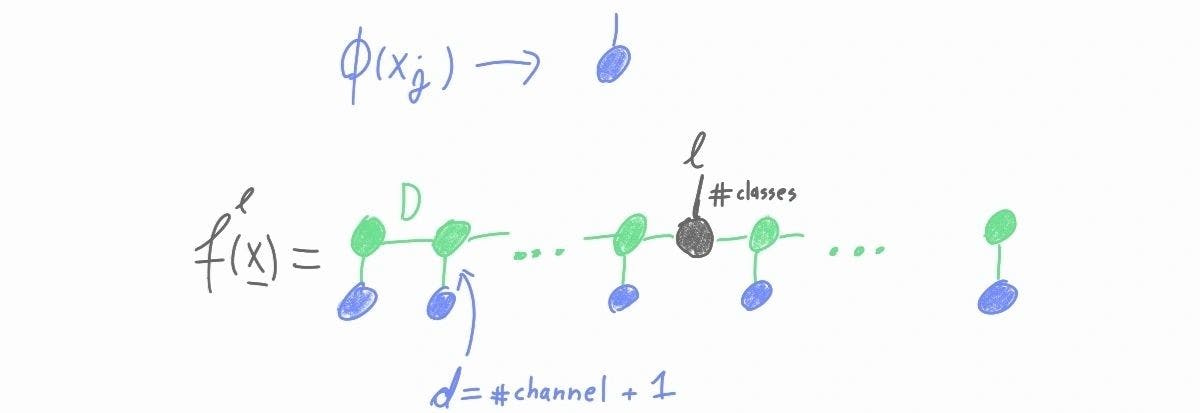
• Embedding: The image is first normalized. After the normalization, each pixel in an image channel has a value between zero and 1/(number of channels). Then the following local feature map is applied to each pixel individually

• MPS model: Each local feature map (blue tensors) is then contracted with an MPS (green tensors). The only remaining tensor with an un-contracted leg is positioned in the middle of the MPS (grey tensor) and determines the logits of the model.

• TI-MPS: In the uniform case, the MPS starts with an auxiliary initial vector (orange tensor). The "logit" tensor is moved to the end of the MPS.

• Loss: as a loss we used the multi-class cross entropy

• Initial condition: The initial condition is chosen such that each of the logits is close to one independent of the input. In particular

Augmentation

We used torchvision.transforms to augment the datasets. We performed hyper-parameter tuning for the given model to improve the various transformation parameters and probabilities. In particular, we used the following sequence of transformations ( Transformation_name(parameter_1, parameter_2,... parameter_n) -- along with parameters in the brackets, we also tuned the probability of applying the change):

• Random pixel shift in the range [-aug_phi, aug_phi]
• Random color jitter: transforms.ColorJitter(brightness=brightness, contrast=contrast, saturation=saturation, hue=hue)
• Random sharpness: transforms.functional.adjust_sharpness(sharpness_factor=sharp_fac)
• Random Gaussian blur: transforms.GaussianBlur(kernel_size=blur_kernel_size)
• Random horizontal flip: transforms.RandomHorizontalFlip()
• Random horizontal flip: transforms.RandomHorizontalFlip()
• Random affine transformation: transforms.RandomAffine(rotate, translate=(txy, txy), scale=(scale_min, scale_max))
• Random perspective transformation: transforms.RandomPerspective(distortion_scale=perspective_scale)
• Resize: this transformation is always applied transforms.Resize(resize)
• Random crop: transforms.RandomCrop(crop)
• Random elastic transformation: (here we used the elasticdeform library as import elasticdeform.torch as etorch ) etorch.deform_grid(displacement)
• Random erasing: transforms.RandomErasing(scale=(erasing_scale_min, erasing_scale_max), ratio=(0.3, 3.3))

The order of transformation is fixed and is the same as given above, independent of the dataset. During hyper-parameter tuning, the training was restricted to a maximum of 30 epochs.

The best parameter set was chosen based on the validation accuracy of the 10-fold cross-validation average. If several parameter configurations had the same average, the one with the smallest train accuracy average was chosen. We expect these cases to have better generalization properties. All tuning runs and evaluation runs with different bond dimensions can be found on the WANDB under projects MNIST_MPS, FashionMNIST_MPS, and CIFAR10_MPS.

Results

Our model is implemented in PyTorch and TensorFlow. Due to the time-consuming graph construction of our implementation of the TensorFlow version, we finally used only PyTorch in our experiments. All implementations can be found on GIT, and all tuning runs can be found on WANDB.

Accuracy

Interestingly we observe that there is no over-fitting even for the largest models (on all considered datasets). We observe that the validation and test accuracies are about 1% larger than the training accuracy during the evaluation phase image transformations. The specific training, validation and testing accuracies during training on the MNIST dataset (D=90) are shown in the following figure.

We evaluated the chosen hyper-parameter setting on models with increasing bond dimensions and on the permuted versions of the datasets.

The final best error rates obtained by an ensemble of MPS models are 0.37% (MNIST), 7.57% (FashionMNIST) and 31% (CIFAR-10). These results significantly improve the MPS existing baselines.

Entropy

Matrix product state classifiers have only one parameter, namely the bond dimension D. In quantum mechanics, the bond dimension determines how well an MPS state represents a given quantum state. Here we ask ourselves, what is the meaning of the entanglement entropy in the discussed classification setting. We would like to know if strong volume-law correlations between pixels prohibit an area-law MPS from achieving good accuracies on classification tasks. For this reason, we also considered the permuted versions of the datasets, which (most likely) exhibit volume law classical and quantum correlations. We would thus expect that the accuracy of permuted datasets is much lower than in their non-permuted versions. However, although there is an accuracy drop on the permuted datasets, it is not very large. A similar accuracy can be achieved with only a slightly larger MPS. This suggests that the bond dimension is not the main limiting factor in training MPS classifiers.

To quantify this observation, we calculate the average entanglement entropy of the MPS over all classes at different bond dimensions. The entanglement entropy follows the accuracy of the MPS. However, it is far from reaching the volume law upper bound of entanglement entropy (see figure below).

Before we continue, we note that an ensemble of MPS models is again an MPS model with a bond dimension that is a sum of bond dimensions of the MPS models in the ensemble. By comparing the accuracy of a small-bond dimension MPS ensemble with a single large-bond dimension MPS model, we observe that the former is larger than the latter. However, the big MPS model has significantly more parameters. On the other hand we see that it has a smaller entropy when compared to the MPS ensembe, where MPS states representing different models are essentially orthogonal. Assuming the orthogonality of MPS states in the ensemble the entropy of an ensemble of the model is given by

These observations hint that our training is still sub-optimal. Perhaps a loss that prefers solutions with a larger entropy rather than "simple" solutions with smaller entropy would improve results.

Conclusions

To conclude. In this post I presented three improved baselines for MNIST, FashionMNIST, and CIFAR10 classification. These improvements have to be taken into account when discussing other possible tensor network models in order to avoid spurious improvements. Also the MPS setting is the clearest to further study the relevance of entanglement entropy in classification tasks.